The solubility of drugs, the taste of chocolate or the solidity of concrete – these are only a few examples of physical or chemical material properties which are influenced by particle size. Hence, the determination and knowledge of the particle size distribution is an essential part of the quality control process for industrial products.
From incoming and production control to research and development, sieve analyses are used to determine a number of parameters or simply the particle size. Easy handling, low investment cost and high accuracy make sieve analysis one of the most frequently used procedures for measuring the particle size. This white paper gives an overview of the different sieving techniques and describes the necessary steps to ensure reliable results.
Sieving is carried out to separate a sample according to its particle sizes by submitting it to mechanical force. The direction, intensity and type of force depends on the chosen sieving method. The sample is either moved in horizontal or vertical direction. Air jet sieving is a special case, here the sample is dispersed by an air jet blown out of a rotating nozzle.
All information here has been provided by Endecotts Ltd experts in the production and sieving apparatus and methodologies.
Which factors need to be established to select a suitable sieving method?
Particle Size
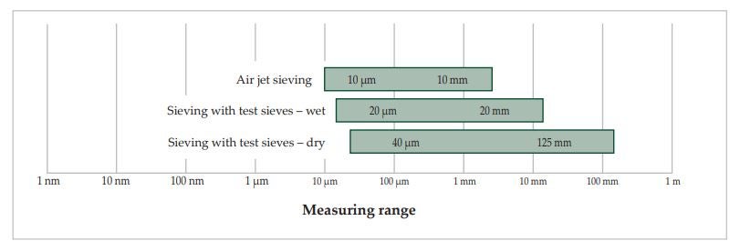
If the required measuring range lies between approximately 40 microns and 125 mm, classical dry sieving is the method of choice. The range may be extended to 20 microns by wet sieving and to 10 microns by air jet sieving.
Sample Properties
It should be taken into account whether the particles form agglomerates, which density the material has or if it tends to be electrostatically charged
Standards
Sieving methods are described in the DIN standard 66165. If industry-specific test procedures or standards exist these also determine the choice of method.
Number of Fractions
Are several fractions required? Or is it sufficient to know which percentage of the sample is smaller or bigger than a defined particle size? The method for obtaining the latter information is called a sieve cut because the sample is simply separated into two fractions.
Different Sieving Methods
Once these questions are satisfactorily answered, a suitable sieving method can be selected. This page describes the different sieving techniques
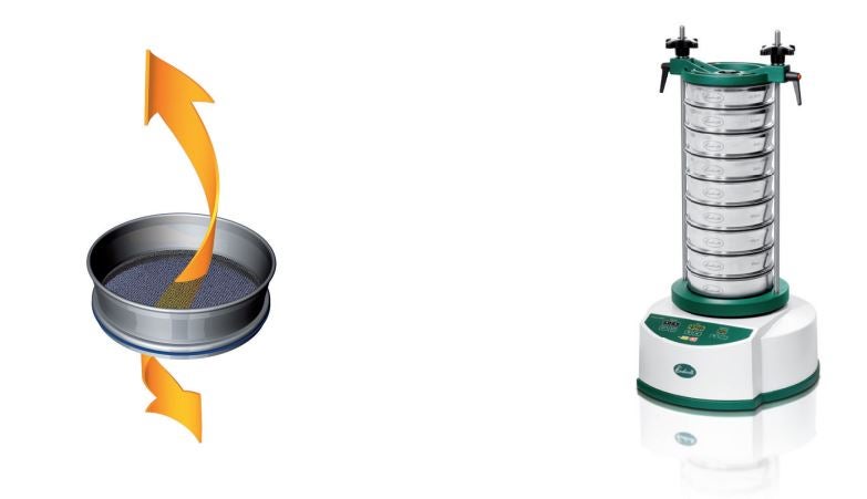
Vibratory sieving: Vibratory sieving submits the sample to three-dimensional movements. A vertical throwing motion is superimposed by a circular movement. This mechanism causes the particles to be evenly distributed over the entire sieving surface and to be thrown into the air where they ideally change their orientation in a way that allows them to be compared to the sieve apertures in all possible dimensions. Vibratory sieve shakers like the OCTAGON 200 (fig. 3), the EFL 300 and TITAN 450 operate according to this principle. All ENDECOTTS vibratory sieve shakers are suitable for dry as well as wet sieving. The OCTAGON 200CL provides reproducible, globally comparable results because it operates indepentdently from the power frequency.
Wet sieving: A special case of vibratory sieving is wet sieving. Agglomerates, electrostatic charging or a high degree of fineness can all make the sieving process difficult and in such cases wet sieving may be called for. This involves washing the sample through the sieve stack in a suitable medium which is usually water.
ENDECOTTS Sieve Shakers Minor 200, OCTAGON 200CL, OCTAGON 200 and TITAN 450 are suitable for wet sieving.
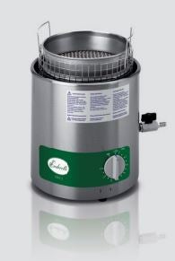
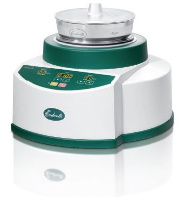
Air jet sieving: To obtain a sieve cut by air jet sieving only one sieve is used instead of a stack of sieves, and the sieve itself is not put into motion. An industrial vacuum cleaner generates low pressure inside the sieve chamber. The sucked-in air escapes with high speed from the rotating slit nozzle below the sieve and disperses the particles which can then be compared to the sieve apertures. When the particles hit the sieve lid they are not only redirected but also deagglomerated. The particles which are small enough are then transported through the sieve mesh and sucked in. It is also possible to collect them in a cyclone. ENDECOTTS offers the Air Sizer 200 for air jet sieving.
Features include adjustable speed from 5 - 55 rpm and automatic vacuum regulation (accessory). The machine may be controlled with the ENDECOTTS SieveWare evaluation software.
Sieve Analysis Step by Step
A complete sieving process consists of the following steps which should be carried out
precisely and carefully.
- Sampling
- Sample division (if required)
- Selection of suitable test sieves
- Selection of sieving parameters
- Actual sieve analysis
- Recovery of sample material (if required)
- Data evaluation
- Cleaning of the test sieves
a) Sampling
Correct sampling is essential to obtain a representative laboratory sample, especially if the material is heterogeneous. Some important questions should be clarified in advance:
- Which quantity is required to ensure representativeness of the original sample
- From which part of the original material should the sample be taken
Some industry-specific standards provide guidelines and directions on the correct sampling process.
A universal rule determines that the volume of the smallest part sample is proportional to the maximum particle size and can be calculated with the following formula:
G [kg] = 0.07 [kg/mm] x z [mm]
which indicates how much sample “G” must be extracted from a bulk sample with maximum particle size “z” to obtain a representative quantity. Taking a coal sample
with a maximum particle size of 5 cm as an example, the following calculation applies:
G [kg] = 0.07 kg/mm x 50 mm
G = 3.5 kg
Consequently, the extracted sample amount should be at least 3.5 kg to make sure it is representative. For other materials than coal, their different densities should be taken into account.
b) Sample Division
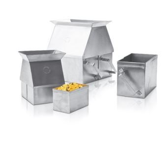
If a sample quantity is too large for analysis, it must be divided with the means of sample dividers (fig. 5) in a way that ensures the part sample represents the original material. Endecotts offer a range of high quality manual sample splitters in order to divide all pourable solids so accurately that the characteristic composition of each fraction of the sample corresponds exactly to that of the original bulk sample.
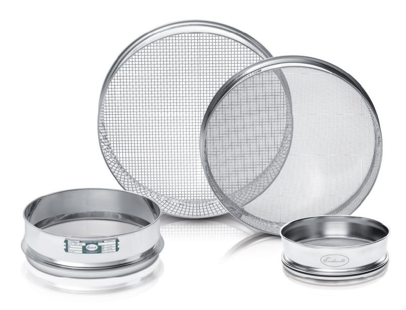
c) Selection of suitable test sieves
The selection of the sieves depends on the sample quantity and on the approximate particle size distribution. To cover the complete particle size range of the sample, the increments of the mesh apertures should follow a logarithmic series. This is frequently done with the help of the Renard series, for example R10/3. The standard DIN 66165 contains some guidelines on the selection of sieve diameters and mesh sizes. It also stipulates the maximum sample load permitted for different mesh sizes and also the maximum particle size.
The maximum sieve oversize permitted on a sieve can be approximately calculated with the formula
R = 0.00178 x D2 x w0.667 x ρ
with R being the maximum permitted sieve oversize in [g]. D stands for the sieve diameter (200 mm / 300 mm etc.), w is the mesh size in [mm - (the value is used in the
formula without unit)] and ρ describes the material density. In the standard 66165 and in the above example a density of 1 kg/dm3 was assumed. The standard also describes
the maximum load per sieve which should not exceed the maximum sieve oversize R by more than twice the amount.
The maximum particle size permitted can be calculated by using this formula xmax = 10 x w0.7 with xmax [mm] being the maximum particle size permitted, and w describing the nominal mesh size of each sieve (the value is used in the formula without unit). For a sample on a sieve with an aperture size of 250 microns the following calculation is used to determine the maximum particle size permitted:
xmax = 10 x w0.7
xmax = 10 x 0.2500.7
xmax = 3.79 (unit = mm)
d) Selecting suitable sieving parameters
Usually, industry-specific standards or company-specific regulations contain information about the required sieving parameters. Should this not be the case, those parameters need to be ascertained by experiment. The sieving time and, when using vibratory sieve shakers also the amplitude, are the most important factors. Observing the maximum sieve load helps protecting the sieve from damages and ensures that every particle has the possibility to compare with the sieve mesh as frequently as possible and in every dimension.
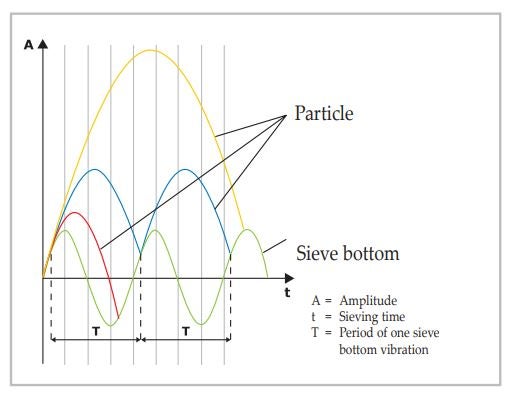
Amplitude:
During a sieving process there is a continuous size comparison between sieve apertures and particles. If a particle is smaller than an aperture, it passes the mesh. If it does not pass the aperture it is thrown upwards with the next lifting of the sieve bottom, takes a different orientation – which is important with longish particles – and hits the mesh again for a new comparison. Each comparison is an opportunity for the particle to pass the sieve mesh. Hence, the objective of a sieving process is to generate as many comparisons as possible in a given time. This is ideally the case when within the period of a sieve bottom vibration exactly one comparison takes place and the particles which do not pass the sieve mesh are accelerated in a way that within the next period another comparison takes place. This state is called statistical resonance (blue curve in fig. 8). If a particle is accelerated too strongly it has only very few occasions to compare with the sieve apertures (yellow curve) and the complete separation of the sample is delayed; if a particle is hardly accelerated or not at all, it cannot orientate freely for a new comparison (red curve). The acceleration rate of a particle depends on the set amplitude. The optimum amplitude for a particular material and quantity needs to be ascertained empirically. Amplitude here means the complete oscillation in the horizontal plane, below as well as above the idle position. An amplitude of 1.2 mm indicates a movement of + 0.6 mm and – 0.6 mm in relation to the idle position.
Sieving time:
According to DIN 66165 the sieving process is considered as finished when, after one minute of sieving, less than 0.1% of the feed quantity passes the sieve. If the undersize is larger the sieving time needs to be extended. Experience has shown that vibratory sieving in 3 dimensions is particularly suitable for achieving a sharp separation of fractions in a very short time.
e) Carrying out the actual sieve analysis
After selection of the parameters, the actual sieving process starts. The following steps have to be carried out in chronological order:
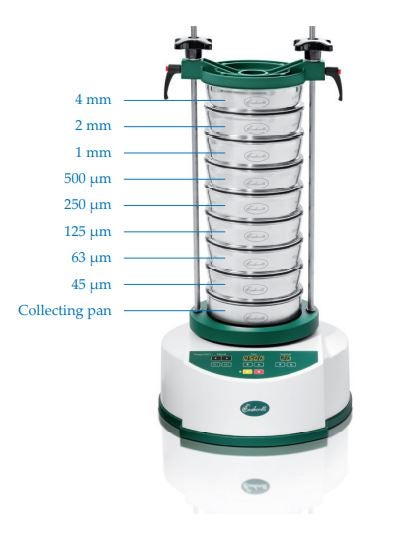
- Put together a sieve stack with collecting pan.
- Select sieving aids, if required: for mesh sizes < 500 microns the use of rubber balls, cubes, chains or brushes is recommended to facilitate passage of the sample. For mesh sizes < 100 µm just light spheres are recommended.
- Determine the empty weight of sieves and collecting pan: This can be done software-based or manually by using a balance. Suitable programs such as SieveWare make weighing and evaluation much easier.
- Place the sieve stack with increasing mesh size on the collecting pan (fig. 9)
- Weigh the sample and put it on the top sieve (biggest mesh size); clamp sieve stack on the machine
- Set the amplitude / speed and sieving time on the sieve shaker
- Start the sieve shaker
- When the sieving time has expired, weigh each sieve and the collecting pan with the fraction on it
- Determine the mass and percentage of each fraction
- Evaluation
f) Recovery of sample
When the sieving process is finished the material is removed from the sieves. The recovery of the fractions is a decisive advantage of sieve analysis over most optical measurement methods. The fractions are not only analytical values but physically exist and can be used for further processes following sieve analysis.
g) Determination and evaluation of data
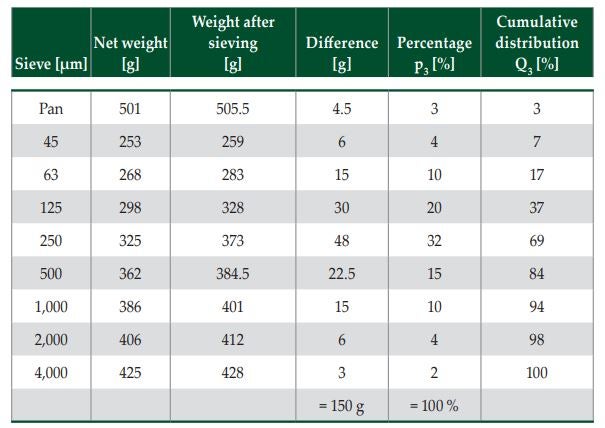
Data evaluation can be done manually or with the help of a software like Endecotts SieveWare. As shown in Table 2 the percentages are calculated and displayed
graphically.
The empty sieves are weighed before and, containing the respective fractions, after the sieving process. The difference corresponds to the weight of each fraction. If these are put into relation to the total weight of the sample the percentage of each fraction can be calculated. This method has the advantage that due to the absence of dimensions sieving is carried out independently of the density or mass of the sample material. The difference between weighed sample and sum of the single fractions is called sieve loss.
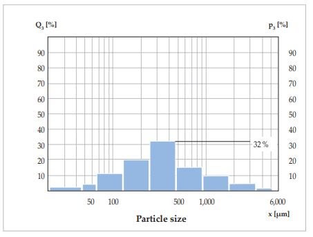
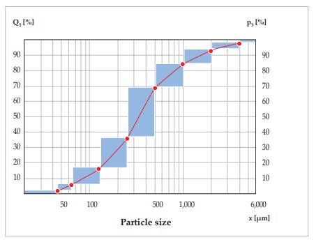
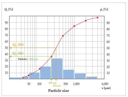
If this is more than 1 % of the feed quantity DIN 66165 stipulates that the sieve analysis needs to be repeated. The mass percentages of the fractions can be graphically displayed as histograms. In the example the largest fractions can be found between 250 microns and 500 microns with 32 %. By adding up the single fractions and through interpolation between the measuring points the cumulative distribution curve Q3 is obtained.
This curve helps to determine a variety of sample properties. Taking a look, for example, at the particle size 250 microns the corresponding value of 36 % can be read off the y-axis. This means that 36 % of the total sample are smaller than 250 microns (fig. 12).
To determine the median Q3 (50) of this distribution, the corresponding particle size (330 microns) is read off the x-axis. This means that 50 % of the sample mass are smaller than or equal 330 microns. In this way various x(Q3 ) or Q3
(x) values can be determined.
A software like SieveWare allows for quick and error-free evaluation of various parameters.
h) Cleaning of test sieves
Test sieves are measuring instruments which should be treated with care before, during and after sieving. By no means should the sample be forced through the sieve mesh during the sieving process. Even a light brushing of the material – particularly through very fine fabric – may lead to changes of the mesh and damage the sieve wire gauze.
Coarser fabrics with mesh sizes larger than 500 microns can be effectively cleaned dry or wet with a hand brush with plastic bristles. Sieves with a mesh size below 500 microns should generally be cleaned in an ultrasonic bath. Drying cabinets of various sizes can be used for drying test sieves which should be placed vertically inside the cabinet. It is recommended not to exceed a temperature of 80 °C. With higher temperatures especially the fine metal wire mesh could become warped; as a result, the tension of the fabric inside the sieve frame is reduced which makes the sieve less efficient.
If deviations from the uniformity of the mesh are observed, the sieve is no longer suitable for quality control purposes (DIN ISO 9000 ff) and must be replaced